Introducing Pivot Tables
If you aren’t aware of pivot tables or haven’t had the time to try out this function in Excel, you need to learn about this powerful feature. Pivot tables provide a way to cross-tabulate, sort, segregate, and aggregate tabular data. Using pivot tables, you can quickly summarize data and extract totals, averages, and other information from the source data.
I first found out about pivot tables when I was working with our business unit financial analyst years ago. She didn’t like our corporate ERP system (SAP) any more than I did, and found it much faster to dump the raw data into Excel and get the answers to her questions by using a pivot table. I’ve been a pivot table convert ever since.
Using the spreadsheet newABCDCatering.xls developed in the last post, let’s add a pivot table and answer the questions raised previously:
- What were the total sales in each of the last four quarters?
- What are the sales for each food item in each quarter?
- Who were the top 10 customers for ABCD Catering?
- Who was the highest producing sales rep for the year?
- What food item had the highest unit sales in Q4?
To build the pivot table, begin by clicking cell A1 pressing Ctrl+* key combination (hold down the Ctrl key and press *). This key combination selects the data in the table while ignoring the blank cells surrounding the table. You can also select the data (with more effort) by selecting cell A1 and scrolling to the last column and row of data while holding down the left mouse key.
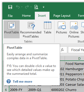
Next, select the Insert tab and click the PivotTable button.
Because you’ve selected the spreadsheet data, the dialog should already be
populated with the range Sheet2!$A1:$M791 as shown below
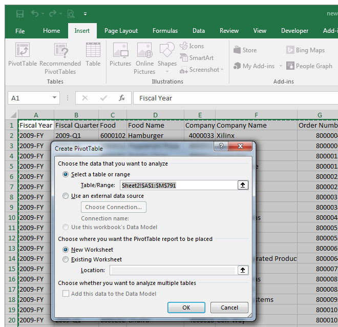
Click OK to create the empty pivot table.
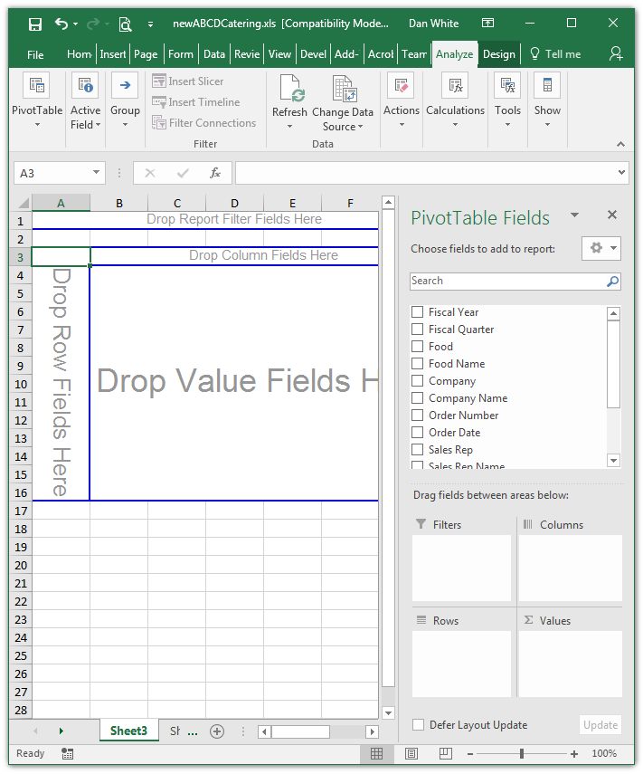
Now you’re ready to do some data analysis.
What were the total sales in each of the last four quarters?
To understand the sales for the last four quarters, create a pivot table with “Fiscal Quarter” as a Row Label, and “Net Booking” as a Values field. To do this, click “Fiscal Quarter” in the list of fields and drag the field to the Row Labels section. Next, click “Net Booking” and drag the field to the Values section.
The spreadsheet updates to show the sum of net bookings for each quarter as shown below.
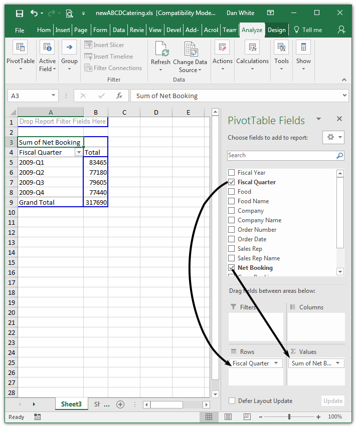
Based on the spreadsheet data, the total net bookings in each of the last four quarters were $83465, $77180, $79605 and $77440 respectively.
What are the sales for each food item in each quarter?
To answer this question, start with “Fiscal Quarter” as a row label and “Sum of Net Bookings” as the value as you did for the previous question. Now, add a column header for “Food Name” by dragging “Food Name” to the Column Labels section. The spreadsheet should now look like this:
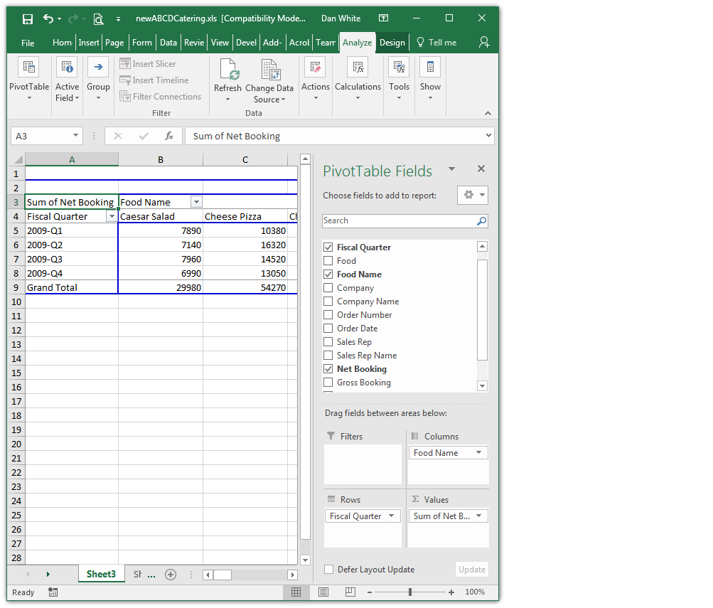
Note that each food item is listed as a column header, each of the four quarters are listed as row headers. Using this table, you can quickly scan the data and understand the sales for each food item. For example, Caesar Salad sales were $7890, $7140, $7960, and $6990 in each of the respective quarters.
Who were the top 10 customers for ABCD Catering?
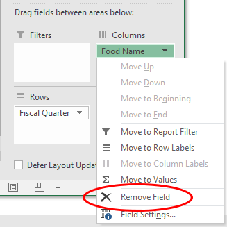
For this question, the “Food Name” and “Fiscal Quarter” data fields and not needed and can be removed by dragging them from the Rows box and the Values box back to the top of the PivotTable Fields panel. Alternatively, click the small triangle next to each field and select “Remove Field” to remove it.
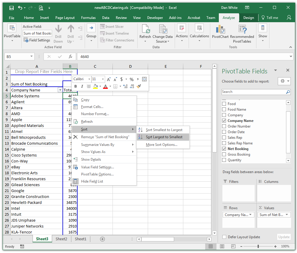
Continue to build the pivot table by dragging the “Company Name” field to the Rows box. The pivot table now contains the list of companies and their purchases, listed in alphabetical order. To find the top 10 customers, select the booking number for Adobe Systems, right-click and choose Sort > Sort Largest to Smallest.
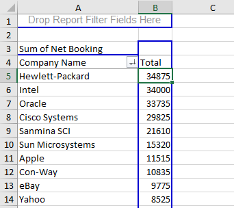
The list is now sorted, the top 10 customers for ABCD Catering are Hewlett-Packard, Intel, Oracle, Cisco Systems, Sanmina SCI, Sun Microsystems, Apple, Con-Way, eBay and Yahoo.
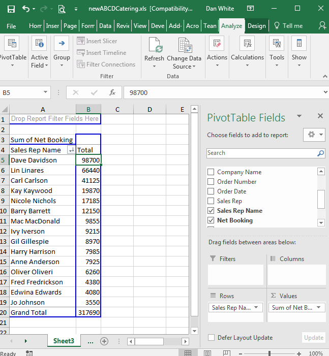
Who was the highest producing sales rep for the year?
At ABCD Catering, sales reps cover multiple accounts. To find the highest producing rep, remove the Company Name field, replace it with the Sales Rep Name field and sort by Net Bookings. The top 10 sales reps are Dave Davidson, Lin Linares, Carl Carlson, Kay Kaywood, and Nicole Nichols.
What are the account assignments for these top reps? To find out, drag the Company Name field into the Row Labels area.
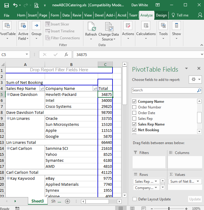
Since Hewlett-Packard, Intel and Cisco Systems were 3 of the top 4 producing accounts, it’s no surprise that their sales rep Dave Davidson was the top performer.
Which food item had the highest unit sales in Q4?
To find the food item with the highest unit sales, remove “Sum of Net Bookings” from the Values box and remove the “Sales Rep Name” and “Company Name” row header fields from the Rows box. Next, drag the Quantity field to the Values box and drag the “Food Name” field to the Rows box.
To filter the table and show only data for 2009-Q4, drag the Fiscal Quarter field to the Report Filter area and select “2009-Q4”. Finally, do a descending sort on the Sum of Quantity field to find the item with the highest unit sales.
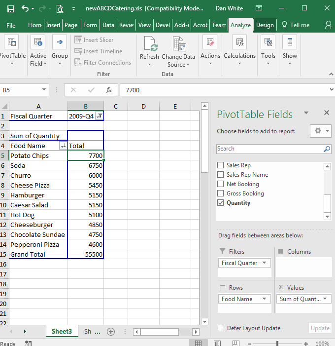
The number one item by unit volume was Potato Chips, followed by Soda and Churro.
These examples should give you a feel for the power and flexibility of pivot tables. In the next post, we’ll automate everything with Python and generate a simple framework for quickly building pivot tables.
Prerequisites
Microsoft Excel (refer to http://office.microsoft.com/excel)
Source Files and Scripts
The spreadsheet newABCDCatering.xls is available at http://github.com/pythonexcels/excelexamples
Originally posted on November 11, 2009 / Updated October 1, 2019